
 AeroSim Docs
Proper Orthogonal Decomposition with Fourier Series
The proper orthogonal decomposition with Fourier series (PODFS) method, as applied to inlet turbulence by Treleaven and others[1], takes the opposite stance to the Synthetic Eddy Method. That method is statistics-prescribed: it builds a fluctuation field to match second-order statistics that the user specifies analytically, and it never needs a precursor. PODFS is data-driven: it records a genuine turbulent field once, compresses it, and replays it at the inlet on demand. What it injects was a real solution of the governing equations, so it carries the true phase organisation and coherent structures that no purely synthetic field can reproduce, and it sits closer to a consistent flow state at the boundary, which is the property that shortens the development fetch.
What PODFS is, and is not
PODFS does not invent turbulence. It records a real turbulent field once, compresses it ruthlessly, and plays it back at the inlet. Its fidelity is therefore bounded by the field it recorded: feed it a poor precursor and it faithfully replays a poor inflow. The guaranteed gains are practical rather than physical - a stored basis several orders of magnitude smaller than the raw recording, and a replay that is continuous, periodic and time-step-independent. The turbulence quality is whatever the precursor had.
Record, compress, replay
See also
The two pieces of mathematics PODFS rests on - proper orthogonal decomposition (an eigenvalue problem on the snapshot correlation) and the Fourier series - are developed from first principles, for readers not already familiar with them, in Mathematical foundations of PODFS.
The method has three stages. A precursor simulation - a separate scale-resolving run whose only job is to produce a long, statistically converged record of turbulence on a plane that matches the intended inlet - is sampled to give a set of \(M\) snapshots of the velocity field on the inlet plane. An offline stage compresses those snapshots into a small basis: a handful of spatial shapes and a few Fourier coefficients per shape. An online stage, running inside the solver, reconstructs the inlet velocity every step from that basis. Only the offline stage is expensive, and it runs once per inflow case.
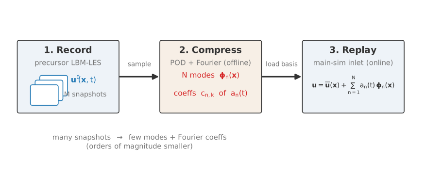
PODFS in three stages. A precursor simulation is recorded as inlet-plane snapshots; proper orthogonal decomposition plus a Fourier-series fit compress them into a few spatial modes and their periodic temporal coefficients; the inlet is then replayed as the mean plus the Fourier-weighted sum of modes. It is a faithful compressor of a recorded flow, not a statistics generator.
Note
Nassu treats the snapshots through a single snapshot-source interface, so the compression machinery never depends on where they came from. A real precursor LES is one source; a synthetic generator that emits snapshots with prescribed statistics is another. Both feed the same compression and replay through this interface, with no change to either. Snapshots are exchanged in the solver’s own plane-export format (a triangulated inlet plane with one field array per recorded step), so recording reduces to an inlet-plane probe and the offline stage reads back exactly what any plane export writes.
Reynolds decomposition
On the inlet plane the recorded velocity is split, as in the other methods, into a time mean and a zero-mean fluctuation,
and the compression is applied to the fluctuation \(\mathbf{u}'\) only, never to the full field. Keeping the mean profile \(\overline{\mathbf{u}}\left(\mathbf{x}\right)\) as a separate object is what later lets the mean velocity and the turbulence intensity be rescaled independently of each other.
Compressing space: proper orthogonal decomposition
POD Lumley[2] answers one precise question: among all possible sets of spatial shape functions, which ordered set reconstructs the most turbulent kinetic energy with the fewest functions? Its answer writes the fluctuation as a sum over modes,
where the \(\boldsymbol{\phi}_{n}\left(\mathbf{x}\right)\) are orthonormal spatial modes - the fixed shapes of the eddies - and the \(a_{n}\left(t\right)\) are scalar temporal coefficients telling how strongly each shape is present at each instant. The sum is truncated to the first \(N\) modes, and that truncation is the spatial compression.
The modes are the eigenvectors of the two-point spatial correlation. With \(M\) snapshots stacked as columns, the method of snapshots Sirovich[3] obtains them from the much smaller \(M\times M\) temporal correlation matrix,
whose eigenvalues \(\lambda_{n}\) are the energy of each mode and whose eigenvectors \(\boldsymbol{\psi}_{n}\) give the temporal coefficients; the spatial modes are recovered by projecting the snapshots onto \(\boldsymbol{\psi}_{n}\). Because the number of snapshots is far smaller than the number of grid points on the inlet plane, the \(M\times M\) problem is far cheaper than the full spatial eigenproblem.
Why POD and not a Fourier transform in space
Fourier modes are fixed sinusoids; they are optimal only for statistically homogeneous directions. An ABL inlet is strongly inhomogeneous in the wall-normal direction, so Fourier modes there waste coefficients. POD modes adapt to the actual flow and are provably the most energy-compact linear basis - a given accuracy is reached with the fewest modes. That energy-compactness is the entire reason POD is used for the spatial step.
The eigenvalues also give a stopping rule. The fraction of energy captured by keeping \(N\) modes is the relative cumulative energy,
and \(N\) is chosen so \(E\left(N\right)\) reaches a target, commonly 90-99% of the resolved fluctuating energy. The discarded modes are the low-energy, high-wavenumber small scales, a point returned to below.
Compressing time: the Fourier-series step
After POD there remain \(N\) temporal signals \(a_{n}\left(t\right)\), each sampled at the \(M\) precursor steps. Storing them raw still ties the inflow to the precursor’s time step and length. The PODFS step represents each coefficient as a truncated Fourier series over the precursor period \(T\),
collapsing each signal to a handful of complex coefficients \(c_{n,k}\). This is what gives the method its three defining properties Treleaven and others[1]: the reconstructed inflow is continuous (it can be evaluated at any instant, not only at stored steps), periodic (it loops seamlessly with period \(T\)), and time-step-independent (the downstream solver may use any \(\Delta t\)). If the precursor turbulence is statistically stationary the coefficients are themselves Fourier modes in time, so the series is the natural representation; in practice the signal is only pseudo-periodic, and enough harmonics are kept to capture its dominant spectral content.
Why this matters specifically for an LBM solver
A lattice-Boltzmann solver runs at a fixed lattice time step tied to the lattice speed of sound, and that step is generally not equal to the precursor time step. With raw stored inflow the precursor signal would have to be interpolated onto the lattice clock every iteration. The Fourier-series representation removes that problem entirely: the closed-form series is evaluated at the exact lattice time, with no stored-data interpolation and no resampling artefacts. This is one of the strongest reasons to prefer PODFS over raw recycled inflow in an LBM context.
Reconstruction at the inlet
The online stage is the assembly of the three pieces. Each step the inlet velocity is
Read left to right: take the fixed mean profile, then for each retained mode evaluate its Fourier series at the current time to get a scalar, multiply by that mode’s fixed spatial shape, and sum. The mean \(\overline{\mathbf{u}}\) and the modes \(\boldsymbol{\phi}_{n}\) are bilinearly interpolated from the precursor analysis plane onto the inlet lattice once at start-up. The analysis plane is decoupled from the inlet: it carries its own structured grid and physical extent, so a precursor recorded at a different resolution or spatial scale (for example a wider precursor plane mapped onto a narrower inlet) is resampled through an affine map of the injection box onto the analysis extent. The interpolation runs independently for every refinement level present at the inlet, and only the cheap scalar Fourier evaluations happen per step, so the cost is negligible against the bulk collision and streaming.
Injecting into the LBM
The reconstruction returns a velocity, but the LBM evolves particle distribution functions, so a velocity inlet is the question of which incoming populations reproduce that velocity as their moments. This is handled by the regularized velocity inlet Latt et al.[4] already used for the other inlets - the same path, not a parallel one - and equivalently a Zou-He construction Zou and He[5]. As with the SEM the inlet density is held at the constant reference value \(\rho=\rho_{0}=1\) (fixing the pressure rather than enforcing a solenoidal field), the rate-of-strain is taken from the inlet velocity by finite differences, the SGS viscosity is evaluated, and the populations are reconstructed. Being a replay of a near-consistent field, PODFS injects a smoother, more mass-consistent inlet than a synthetic generator; a strictly solenoidal correction is neither required nor exactly representable under the weakly compressible LBM Krüger et al.[6].
The one step that is easy to get wrong is the unit conversion, because the precursor and the basis live in physical units while the solver runs in lattice units. Two independent linear knobs handle it. The velocity is rescaled by vel_mul, a single linear factor applied to the whole reconstructed velocity, mean and fluctuation together, so the turbulence-intensity ratio \(I_{\alpha}=\sigma_{\alpha}/\bar{u}\) is unchanged. The time fed to the Fourier series is rescaled by time_rescale, a factor \(s\) that maps the basis temporal axis onto the solver clock by evaluating equation (6) at an effective time \(t_{\mathrm{eff}}=s\,t_{\mathrm{lat}}\), equivalently a period \(T_{\mathrm{eff}}=T/s\); the period and harmonic frequencies are pre-converted once at setup.
Two knobs, two distinct symptoms
A velocity-units error and a time-units error fail differently and are diagnosed separately. A wrong vel_mul scales the turbulence intensity while leaving the spectral shape in place. A wrong time_rescale shifts every injected frequency, so the development rate and the spectra come out wrong while the intensity may look right. If the injected intensity is correct but the flow develops too fast or too slow, suspect the time conversion before the modes.
As with the SEM, the fluctuation can be confined to a sub-region of the inlet plane through the same domain_limits_yz box: inside it the inlet carries the mean plus the PODFS fluctuation, and outside it the mean velocity only.
The record-compress steps - sampling the precursor plane and turning it into the POD-Fourier basis - are done offline, outside the solver, by the nassu podfs-build command, which writes a single self-describing basis file holding the mean, the POD modes, the Fourier coefficients, the analysis-grid coordinates, and an optional calibrated high-frequency supplement. The solver is load-only: it reads that file and replays it at the inlet, making no POD decisions at runtime.
The high-frequency tail
Both truncations discard high-frequency content. The \(N\)-mode POD truncation drops the low-energy, high-wavenumber modes - the small scales of the dissipation range - which is a documented weakness of POD truncation Berkooz et al.[7], and the \(K\)-harmonic Fourier truncation drops the high-temporal-frequency content of each coefficient. The injected field can therefore look energetic at the large scales while being deficient in the spectral tail.
Key idea
The fix is not to inflate \(N\). Restoring the dissipation range by adding POD modes means carrying hundreds of weak modes for a tiny energy gain. The standard approach is to measure the residual spectrum - the precursor one-point spectrum minus the spectrum of the truncated reconstruction, per component - and, where it is deficient, to add a small synthetic high-frequency supplement calibrated to exactly that residual. The supplement is a cheap, band-limited, per-node-decorrelated fluctuation (filtered noise or random Fourier modes in the spirit of Kraichnan[8] and Klein et al.[9]); being small-scale it is naturally low in coherence, so it fills the tail without disturbing the resolved large-scale statistics. It is optional and calibrated from the residual, not a free parameter.
Tuning the statistics
Because POD is applied to the fluctuation alone, a recorded basis can be reused at a slightly different operating point, but the safe operations are narrower than they look. Rescaling the mean profile is free: \(\overline{\mathbf{u}}\left(\mathbf{x}\right)\) is an independent object and may be scaled or replaced without touching the modes. A uniform turbulence-intensity change is also safe: multiplying every temporal coefficient by one constant factor \(\alpha\) scales the kinetic energy by \(\alpha^{2}\) and leaves the spatial coherence and spectral shape untouched, because a global scalar factors out of the orthonormal modes. Non-uniform rescaling is where the freedom ends - scaling different modes or different components by different factors changes the relative mode energies, which alters the coherence and the spectrum; it is a retargeting of the physics, not a change of amplitude, and must be re-validated. For genuinely different inflow regimes the correct route is a separate basis from a separate precursor per category; modes from different decompositions are not mutually orthogonal, so bases must never be blended.