Synthetic Eddy Method

The synthetic eddy method (SEM) builds a transient turbulent inlet. It was first introduced by Jarrin et al.[1] and presented in an LBM framework by Buffa et al.[2]. It requires the user to provide the flow average velocity profile \(\bar{u}_{\alpha}\) and Reynolds stress tensor \(R_{\alpha\beta}\) associated to the desired turbulent intensity \(\left\{I_{u},I_{v},I_{w}\right\}\). That way, it is possible to reproduce atmospheric boundary layer profiles at inlet.

The idea behind the SEM is physically intuitive. Rather than try to write down a turbulent velocity field analytically, it builds one from a population of moving lumps of vorticity, the eddies, each a small region of correlated motion. The flow seen at the inlet plane at any instant is the combined imprint of all the eddies that happen to overlap it at that moment. Because the eddies are advected with the flow and have a finite size, the field they produce is correlated in space and time, which is exactly the property that lets the turbulence survive downstream rather than dissipate immediately. The user does not place the eddies by hand: they only prescribe the target statistics, and the method seeds and scales the eddies so that the resulting field reproduces those statistics on average.

Warning

Why finite-size eddies and not random noise: persistence. Adding uncorrelated random noise to the mean profile matches the prescribed variances at the inlet plane itself, but it carries no coherent structure, so it dissipates within a short fetch and the flow re-laminarises long before it reaches the model Jarrin et al.[1]. The whole point of advecting finite eddies is that the resulting field is correlated in space and time and therefore survives the journey to the region of interest. A field that matches the inlet statistics but relaminarises downstream is the trap to avoid.

Each user input has a concrete physical meaning:

• The mean velocity profile \(\bar{u}_{\alpha}\left(z\right)\) is the deterministic backbone of the inflow, the time-averaged wind at each height. For the ABL it is the logarithmic profile, and it is added directly to the synthetic fluctuation in equation (1).

• The Reynolds stress tensor \(R_{\alpha\beta}\left(z\right)\) encodes the strength and anisotropy of the turbulence: its diagonal entries are the component variances \(\sigma_{u}^{2},\sigma_{v}^{2},\sigma_{w}^{2}\) (hence the turbulence intensities), and its off-diagonal entries carry the momentum-flux correlations such as \(\overline{u'w'}\) that characterise a sheared boundary layer.

• The Cholesky factor \(A_{\alpha\beta}\), defined in equation (3), is the matrix square root of \(R_{\alpha\beta}\). It is the device that turns the raw, unit-variance eddy field \(\tilde{u}_{\beta}\) into one with exactly the prescribed variances and cross-correlations, so the correct statistics are imposed by construction rather than tuned.

• The length scale \(L\) is the radius of influence of an eddy, that is the integral length scale of the synthesised turbulence. Larger \(L\) produces larger, more persistent eddies.

• The eddy density, through the count \(N\) and the effective count \(N_{\mathrm{eff}}\), controls how many eddies overlap a given point. It must be large enough that the superposition is statistically smooth and approximately Gaussian, matching the near-Gaussian fluctuations of real turbulence.

Key idea: the Cholesky factor imposes the statistics by construction

The eddy superposition \(\tilde{u}_{\beta}\) of equation (4) is a raw, unit-variance, isotropic field; on its own it knows nothing of the target turbulence. The Cholesky factor \(A_{\alpha\beta}\) of equation (3) is the matrix square root of the Reynolds-stress tensor, and multiplying the raw field by it stamps the prescribed variances and cross-correlations onto the output, \(\overline{u'_{\alpha}u'_{\beta}}=K^{2}R_{\alpha\beta}\), where \(K\) is the optional intensity-trim factor introduced below; with \(K=1\) the target \(R_{\alpha\beta}\) is recovered exactly. This is the heart of the method: the correct second-order statistics are imposed by construction, not tuned by trial and error. Everything else - eddy size, count, advection - exists to give \(\tilde{u}_{\beta}\) the right spatial and temporal correlation before \(A_{\alpha\beta}\) sets its amplitude.

Note

The input data for the SEM can be obtained from experimental wind tunnel data or by performing a precursor simulation that reproduces a wind tunnel configuration necessary to generate the wind profile of the desired terrain category. The two routes are interchangeable from the solver’s point of view: both supply the mean profile and the Reynolds-stress tensor that the SEM consumes.

In the SEM, \(N\) synthetic eddies are distributed in random positions \(\left\{x_{i},y_{i},z_{i}\right\}\) in a virtual domain as illustrated below:

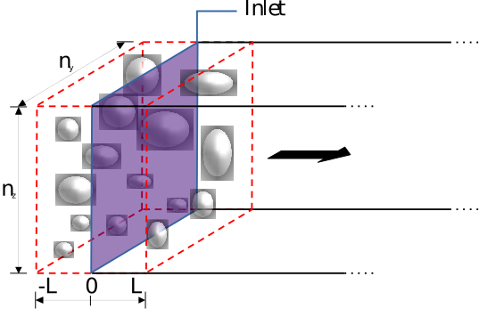
The variable \(L\) is a representative length scale provided as input data that represents the radius of influence of each eddy. That way, the interval to which eddies will be distributed in \(x\) is \(\left[-L,L\right]\), in \(y\) is \(\left[0-L,n_{y}+L\right]\), and in \(z\) is \(\left[0-L,n_{z}+L\right]\). The inlet of the simulation domain is then given by the velocity field in the plane \(x=0\). There, the velocity is given by:

(1)\[ u_{\alpha}\left(0,y,z\right) = \bar{u}_{\alpha}\left(z\right) + {u}'_{\alpha}\left(0,y,z,t\right) \]

where \(u'\) is a fluctuation velocity responsible for providing turbulent intensity at the inlet. This vector field is calculated as:

(2)\[ u'_{\alpha}\left(x,y,z,t\right)=A_{\alpha\beta}\left(z\right)\tilde{u}_{\beta}\left(x,y,z,t\right) \]

in which, \(A_{\alpha\beta}\) is the Cholesky decomposition of the prescribed Reynolds stress tensor with a user defined scaling factor \(K\), introduced by Buffa et al.[2] as a tuning parameter for turbulent intensity:

(3)\[\begin{split} A_{\alpha\beta} = K\left( \begin{matrix} \sqrt{R_{11}} & 0 & 0 \\ R_{21}/A_{11} & \sqrt{R_{22}-A_{21}^{2}} & 0 \\ R_{31}/A_{11} & \left(R_{32}-A_{21}A_{31}/A_{22}\right) & \sqrt{R_{33}-A_{31}^{2}-A_{32}^{2}} \end{matrix} \right) \end{split}\]

and \(\tilde{u}_{\beta}\) is given by:

(4)\[ \tilde u_{\beta}\left(x,y,z,t\right) = \frac{1}{\sqrt{N_{\mathrm{eff}}}}\sum_{i=1}^{N}\epsilon_{i\beta}f\left(\frac{x-x_{i}}{L}\right)f\left(\frac{y-y_{i}}{L}\right)f\left(\frac{z-z_{i}}{L}\right) \]

where \(N_{\mathrm{eff}}\) is the effective number of vortices acting at a domain position, considering \(L\) as a radius of action. It can be calculated with:

(5)\[ N_{\mathrm{eff}} = \left(\frac{N}{2L\left(n_{y}+2L\right)\left(n_{z}+2L\right)}\right)\frac{4}{3}\pi L^{3} \]

Where \(n_{y}\) and \(n_{z}\) are the domain size in \(y\) and \(z\).

Note

The use of \(N_{\mathrm{eff}}\) is an adjustment developed in the current solver, in Buffa et al.[2] the value \(N\) is used instead.

The function \(f\left(x\right)\) is a gaussian function:

(6)\[ f\left(x\right)=2\mathrm{exp}\left(\frac{-1}{2\left(0.225\right)^{2}}x^{2}\right) \]

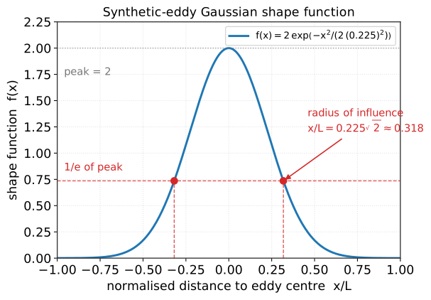
The synthetic-eddy shape function \(f(x) = 2 \exp\!\left(-x^2 / (2 (0.225)^2)\right)\). Each eddy imprints this compact bell on the inlet plane; its width sets the radius of influence, scaled by the integral length scale \(L\). The fast decay is why many overlapping eddies are needed for a statistically smooth field.

The sign tensor \(\epsilon_{i\beta}\) (dimension \(N \times 3\), with eddy index \(i=1,\dots,N\) and direction \(\beta\in\left\{x,y,z\right\}\), as in equation (4)) is composed of random signs \(-1\) or \(+1\) for the directions of each eddy. The evolution of inlet boundary occurs through the displacement of the eddies positions. They move alongside flow direction with the average inlet velocity \(U_{\infty}\), hence:

(7)\[ x_{i}\left(t+\Delta t\right) = x_{i}\left(t\right) + U_{\infty}\Delta t \]

When \(x_{i}\left(t+\Delta t\right)>L\) the eddy is recycled: its streamwise position is wrapped back into the box as \(x_{i}\left(t+\Delta t\right)-2L\), and its cross-stream positions \(y_{i}\) and \(z_{i}\) together with its signs \(\epsilon_{i\beta}\) are re-randomized. The average flow velocity \(U_{\infty}\) is given by:

(8)\[ U_{\infty}=\frac{1}{n_{z}}\int_{0}^{n_{z}}\bar{u}\left(z\right)dz \]

Following the above approach, it is possible to produce a transient velocity field whose statistics return the input data of average velocity and Reynolds stress tensor. Knowing the velocity field at \(x\), the rate-of-strain \(S_{\alpha\beta}\) is calculated through a finite difference scheme and the density is held at the constant reference value \(\rho=\rho_{0}=1\), which fixes the inlet pressure as well. For the obtained \(S_{\alpha\beta}\), the SGS viscosity can be calculated and from all known macroscopic variables, the populations at inlet can be built within the LBM framework.

Note

In finite volume methods one also finds inlet formulations that impose a zero normal density gradient \(\partial \rho/ \partial \mathbf{n}=0\). As reported by Buffa et al.[2], however, the LBM corresponds to a weakly compressible flow, so a purely solenoidal inlet condition is not appropriate and the inlet density must be held fixed to minimize the radiated noise.

Why the density is held constant

This caveat is worth understanding rather than accepting on faith, because it is a direct consequence of the solver’s physics. The LBM does not solve the strictly incompressible equations; it is a weakly compressible method in which pressure and density are tied together. When a synthetic velocity field with non-zero divergence is injected, the solver reads the local imbalance of mass flux as a local change in density, and that density perturbation propagates outward as a spurious acoustic wave. Letting the inlet density float with the synthetic field would therefore inject a steady stream of pressure noise into the domain.

One way to relieve this is to relax the inlet pressure, imposing a zero normal pressure gradient \(\partial p/\partial \mathbf{n}=0\); in Nassu that route was tried and did not behave well in practice. The condition actually used is the simpler one: the inlet density, and with it the pressure, is held at the constant reference value \(\rho=\rho_{0}=1\). This does not enforce exact incompressibility at the inlet, so the residual divergence of the synthetic field still radiates a small disturbance, but that disturbance is acceptable and far smaller than the noise from a floating inlet density. The trade-off is appropriate precisely because the underlying solver is only weakly compressible Buffa et al.[2].

Connection to ABL terrain categories

In wind engineering the upstream terrain is classified into roughness categories, from open sea and flat farmland through suburbs to dense city centres, each with a characteristic roughness length \(z_{0}\) and, with it, a characteristic mean profile, turbulence-intensity profile and length-scale distribution. The SEM is the bridge between such a terrain category and the simulation: selecting a category fixes the target \(\bar{u}_{\alpha}\left(z\right)\) and \(R_{\alpha\beta}\left(z\right)\), and the SEM then reproduces an inflow consistent with that terrain. The targets themselves come either from a wind-tunnel database or from a precursor simulation that builds the desired profiles.

---

[1] (1,2)

Nicolas Jarrin, Sofiane Benhamadouche, Dominique Laurence, and Robert Prosser. A synthetic-eddy-method for generating inflow conditions for large-eddy simulations. International Journal of Heat and Fluid Flow, 27(4):585–593, 2006.

[2] (1,2,3,4,5)

Elisa Buffa, Jérôme Jacob, and Pierre Sagaut. Lattice-boltzmann-based large-eddy simulation of high-rise building aerodynamics with inlet turbulence reconstruction. Journal of Wind Engineering and Industrial Aerodynamics, 212:104560, 2021.