From thermodynamics to the energy equation

This page builds the thermal counterpart to mass and momentum. The LBM chapter recovers continuity and Navier-Stokes from the lattice; here we add the third conservation law, energy, and then show why the production solver does not have to solve it in full. The goal is intuition, not a textbook derivation: where each term comes from, and which terms survive in the low-Mach, small-temperature-difference regime Nassu targets.

The first law, internal energy and enthalpy

Thermodynamics enters fluid mechanics through the first law: the internal energy of a fluid parcel changes by the heat added to it and the work done on it. Per unit mass, with specific internal energy \(e\),

(1)\[ \mathrm{d}e = \delta q - p\, \mathrm{d}(1/\rho) \]

where \(\delta q\) is the heat per unit mass and \(-p\,\mathrm{d}(1/\rho)\) is the compression work (\(1/\rho\) is the specific volume). For a calorically perfect fluid the internal energy is set by temperature alone, \(e = c_v T\), with \(c_v\) the specific heat at constant volume. It is often more convenient to use the enthalpy \(h = e + p/\rho\), which for the same fluid is \(h = c_p T\) with \(c_p\) the specific heat at constant pressure; the two heat capacities differ by the work of expansion, \(c_p - c_v = R\) for an ideal gas.

The thermal moment of the distribution function

In the kinetic picture of the primer, density is the zeroth velocity moment of \(f\) and momentum the first. The internal energy is the trace of the second central moment: it measures the spread of molecular velocities about the mean flow, \(\rho e = \tfrac{1}{2}\int f\,|\boldsymbol{\xi} - \boldsymbol{u}|^2\,\mathrm{d}^3\xi\). Temperature is therefore a genuine kinetic quantity, on the same footing as \(\rho\) and \(u_\alpha\), not an external field bolted onto the flow.

The compressible energy equation

Conservation of energy for a Newtonian fluid, written for the temperature field, sits alongside continuity and the momentum (Navier-Stokes) equation as the third member of the governing set:

(2)\[ \rho\, c_p \left( \partial_t T + u_\alpha \partial_\alpha T \right) = \partial_\alpha\!\left( k\, \partial_\alpha T \right) + \beta_T\, T \left( \partial_t p + u_\alpha \partial_\alpha p \right) + \Phi + S \]

Reading the terms left to right: the left-hand side is the material rate of change of temperature carried by the flow; \(\partial_\alpha(k\,\partial_\alpha T)\) is conduction with thermal conductivity \(k\); the pressure-work term (with \(\beta_T\) the thermal expansion coefficient) couples temperature to compression; \(\Phi\) is viscous dissipation (the heat generated by friction); and \(S\) collects volumetric heat sources, for instance a burner. This is the equation a fully compressible thermal solver integrates, and it is two-way coupled to momentum through both the pressure field and the temperature dependence of the density.

The low-Mach and Boussinesq reductions

Three of those terms are negligible in the regime Nassu targets, and dropping them is what turns the energy equation into something the LBM can carry cheaply.

• Viscous dissipation \(\Phi\) scales with the Eckert number, \(\mathrm{Ec} = U^2 / (c_p\,\Delta T)\), which is tiny at low speed: the heat generated by friction is irrelevant next to the heat the flow is actually transporting.

• Pressure work scales with the Mach number squared; in the weakly-compressible LBM regime (\(\mathrm{Ma} < 0.1\)) it is negligible, so temperature decouples from the acoustic pressure.

• Density variation is dropped everywhere it appears as inertia. This is the Boussinesq approximation He et al.[1], Guo et al.[2]: \(\rho\) is replaced by a constant reference \(\rho_0\) in continuity, in the inertia of the momentum equation, and in \(\rho\,c_p\) above; the temperature dependence of density is retained in one place only, the gravity term, where it produces buoyancy.

With these reductions the energy equation collapses to a plain advection-diffusion equation for temperature,

(3)\[ \partial_t T + u_\alpha \partial_\alpha T = \kappa\, \nabla^2 T + S, \qquad \kappa = \frac{k}{\rho_0\, c_p} = \frac{\nu}{\mathrm{Pr}} \]

with thermal diffusivity \(\kappa\) and Prandtl number \(\mathrm{Pr} = \nu / \kappa\). The only surviving coupling back to the fluid is the buoyancy body force, formed from the temperature deviation from the reference:

(4)\[ F^{\text{buoy}}_\alpha = -\rho_0\, \beta\, (T - T_{\text{ref}})\, G_\alpha \]

with \(\beta\) the thermal expansion coefficient and \(G_\alpha\) the gravitational acceleration vector (pointing along gravity, so the minus sign makes a warm parcel rise). The hydrostatic part is absorbed into the pressure by subtracting \(T_{\text{ref}}\) before forming the force.

Why Nassu transports temperature as a scalar

Equation (3) is exactly the advection-diffusion equation the scalar transport solver already integrates with its own DDF lattice. So in the production route temperature is not a new physics module: it is a passive scalar with diffusivity \(\kappa = \nu/\mathrm{Pr}\), plus the single buoyancy force (4) added to the fluid’s Guo body force. The fluid collision operator is untouched and the equilibrium uses the constant reference density \(\rho_0\). The full energy equation (2), with its pressure work and dissipation, only returns on the compressible LBM path.

The variable-density limit beyond Boussinesq

The Boussinesq reduction holds only while \(\beta\,\Delta T \ll 1\). When the temperature difference is large enough to change the density by an appreciable fraction, the step of freezing \(\rho\) in the inertia is no longer admissible, yet acoustics may still be negligible. The intermediate reduction that keeps the density variation while filtering the acoustics is the low-Mach limit: the pressure is split into a spatially uniform thermodynamic part \(P\), held fixed in time for an open domain (\(\mathrm{d}P/\mathrm{d}t = 0\)), and a hydrodynamic part that drives the flow. The density is then slaved to temperature through the equation of state,

(5)\[ \rho = \frac{P}{r\,T}, \]

and the buoyancy term keeps its exact form \((\rho - \rho_\infty)\,G_\alpha\), of which the Boussinesq force (4) is the linearization \(\rho - \rho_\infty \approx -\rho_0\,\beta\,(T - T_{\text{ref}})\) for small \(\Delta T\). The energy equation (2) is retained as an enthalpy transport with conduction at a real Prandtl number, but its pressure-work and dissipation terms still drop in the low-Mach limit. This is the closure required for strongly buoyant, fire-scale flows; its place in the model is set out on the thermal modeling hierarchy page.

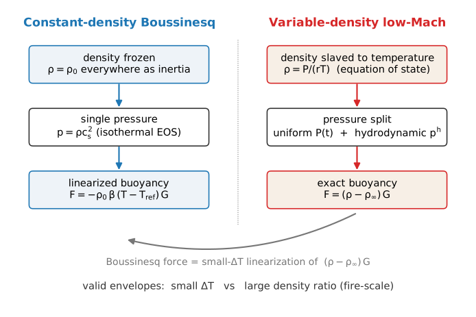
Boussinesq versus variable-density modelling of the same buoyant flow. The Boussinesq route freezes the density at a reference \(\rho_0\) and couples temperature back through a single linearized buoyancy force; the variable-density low-Mach route slaves the density to temperature through the equation of state \(\rho = P/(rT)\), splits the pressure into a uniform thermodynamic part \(P(t)\) and a hydrodynamic part \(p^h\), and keeps the buoyancy exact. The Boussinesq force is the small-\(\Delta T\) linearization of the exact \((\rho - \rho_\infty)\,G\).

The enthalpy form the variable-density solver integrates

The low-Mach closure above retains the energy equation as enthalpy transport. The production variable-density route makes that concrete: it transports the specific enthalpy \(h\), not the bare temperature \(T\). With a calorically perfect fluid and a constant specific heat \(c_p\), the two are related by a linear caloric law referenced to a datum \(h = 0\) at \(T_{\text{ref}}\),

(6)\[ T = T_{\text{ref}} + \frac{h}{c_p}, \qquad \mathrm{grad}\,T = \frac{1}{c_p}\,\mathrm{grad}\,h . \]

The energy equation is the single-species, variable-density low-Mach form of Taha et al.[3]: the material derivative of enthalpy balances conduction and a volumetric heat release,

(7)\[ \rho\,\frac{\mathrm{D}h}{\mathrm{D}t} = \partial_\alpha\!\left( \lambda\, \partial_\alpha T \right) + Q, \qquad \frac{\mathrm{D}h}{\mathrm{D}t} = \frac{1}{\rho}\left[\, \partial_\alpha\!\left( \lambda\, \partial_\alpha T \right) + Q \,\right], \]

with \(\lambda\) the thermal conductivity and \(Q\) a volumetric heat-release rate (energy per unit volume per unit time, lattice units). The pressure-work and viscous-dissipation terms have already dropped in the low-Mach, small-Eckert-number limit, so no \(\mathrm{D}p/\mathrm{D}t\) or \(\Phi\) appears.

Advection in non-conservative form

The advective part of the material derivative is carried in non-conservative (primitive) form, \(u_\alpha \partial_\alpha h\), discretised by first-order upwinding. In the smooth, shock-free low-Mach regime Nassu targets, the non-conservative and conservative forms recover the same macroscopic equation, so the choice is one of discretisation robustness rather than physics Wissocq and Sagaut[4]. The conservative form earns its keep only across discontinuities, which the acoustically filtered low-Mach flow does not develop.

Conduction as variable-coefficient enthalpy diffusion

Conduction is written directly on the enthalpy. Taking the thermal conductivity at a real Prandtl number,

(8)\[ \lambda = \frac{c_p\, \mu(T)}{\mathrm{Pr}}, \]

and substituting \(\mathrm{grad}\,T = \mathrm{grad}\,h / c_p\) from (6), the \(c_p\) cancels and the conduction term becomes a diffusion of enthalpy with coefficient \(D = \lambda / c_p = \mu(T)/\mathrm{Pr}\),

(9)\[ \partial_\alpha\!\left( \lambda\, \partial_\alpha T \right) = \partial_\alpha\!\left( \frac{\mu(T)}{\mathrm{Pr}}\, \partial_\alpha h \right) = \partial_\alpha\!\left( D\, \partial_\alpha h \right) . \]

The effective thermal diffusivity that actually advances \(h\) is therefore

(10)\[ \alpha_{\text{eff}} = \frac{\lambda}{\rho\, c_p} = \frac{\mu(T)}{\rho\,\mathrm{Pr}} . \]

This is the central change from the Boussinesq route. There the diffusivity is the single frozen compile-time constant \(\kappa = \nu/\mathrm{Pr}\) of (3). Here \(\alpha_{\text{eff}}\) is a field: it varies because the density is slaved to temperature through the equation of state \(\rho = P/(rT)\) (5), and optionally because the viscosity itself depends on temperature.

The viscosity law

The dynamic viscosity \(\mu(T)\) defaults to a constant \(\mu_0\). An optional power law \(\mu(T) = \mu_0\,(T/T_{\text{ref}})^{n}\) is available, matching the form Taha et al.[3] use for their methane fire. The reference value \(\mu_0\) defaults to the molecular dynamic viscosity at the reference state, \(\nu_0 = (\tau - 1/2)/3\) in lattice units, so that with constant \(\mu\) and constant \(\rho\) the coefficient \(\alpha_{\text{eff}}\) reduces to the frozen \(\nu_0/\mathrm{Pr}\) of the Boussinesq route.

The conservative face-flux discretisation

A spatially varying diffusion coefficient is discretised in conservative face-flux form, the standard treatment for variable-coefficient diffusion. The discrete operator at a node sums, over each lattice axis \(d\), the net flux through the two faces normal to that axis,

(11)\[ \partial_\alpha\!\left( D\, \partial_\alpha h \right) \;\longrightarrow\; \sum_{d}\Big[\, D_{d+1/2}\,(h_{d+1} - h_{d}) \;-\; D_{d-1/2}\,(h_{d} - h_{d-1}) \,\Big], \]

with the face-averaged coefficient taken as the arithmetic mean of the two adjacent node values,

(12)\[ D_{d\pm 1/2} = \tfrac{1}{2}\,( D_{\text{node}} + D_{\text{neighbour}} ), \qquad D = \frac{\mu(T)}{\mathrm{Pr}}, \]

where each node’s \(D\) is evaluated locally from its temperature through the viscosity law \(\mu(T)\). Defining the coefficient on faces from the two flanking nodes makes the flux leaving one cell equal the flux entering its neighbour, so enthalpy is conserved to machine precision in the interior.

The volumetric heat source

The source term in (7) is a volumetric heat-release rate \(Q\) (energy per unit volume per unit time, lattice units). The source_regions.rate input sets \(Q\) rather than a temperature rate: the update adds \(Q/\rho\) to \(\mathrm{D}h/\mathrm{D}t\), consistent with the \(\rho\,\mathrm{D}h/\mathrm{D}t = \ldots + Q\) balance, so a fixed burner power deposits the same enthalpy regardless of the local density.

Viscous dissipation is dropped

The viscous-dissipation heating \(\Phi\) in the full energy equation (2) is dropped. It scales with the Eckert number and is negligible at the low Mach and low Eckert numbers of buoyant CWE and fire-scale flows, the same argument that removes it from the low-Mach reduction.

The Eckert number \(\mathrm{Ec} = U^2/(c_p\,\Delta T)\) is a ratio: it weighs frictional heating against the imposed temperature difference, not its absolute size. For a buoyant or fire-scale case with a genuine \(\Delta T\) of several to tens of kelvin it is tiny (\(\mathrm{Ec}\lesssim 10^{-2}\)) and the drop is exact. But if energy is added to an essentially isothermal run purely for a more complete field, \(\Delta T \to 0\) and \(\mathrm{Ec}\to\infty\), so the ratio argument no longer applies. What still justifies the omission there is the absolute bound on frictional heating, the recovery-temperature rise \(U^2/(2 c_p)\): for air at CWE wind speeds this is sub-kelvin (about \(0.05\) K at \(10\) m/s, \(0.45\) K at \(30\) m/s) and dynamically inert through buoyancy. Viscous dissipation therefore matters only outside this regime - at high Mach, at high Brinkman number \(\mathrm{Br} = \mathrm{Ec}\,\mathrm{Pr}\), or when a sub-kelvin temperature signal is itself the quantity of interest.

Stability: the hottest cell sets the diffusion limit

Because \(\alpha_{\text{eff}} = \mu(T)/(\rho\,\mathrm{Pr})\) (10) carries \(\rho\) in the denominator, it is largest in the hottest, lowest-density cells. The explicit finite-difference diffusion number must respect the usual bound everywhere, which means it is tightest there:

(13)\[ \frac{\alpha_{\text{eff}}\,\Delta t}{\Delta x^{2}} \le \frac{1}{2\,\mathrm{dim}} \quad\text{in the hottest cell}, \]

with \(\mathrm{dim}\) the spatial dimension. A run that is stable at the reference state can still violate (13) once a region heats up and its density drops, so the limit must be checked against the peak expected temperature, not the mean.

Where this leaves us

The thermodynamic foundation reduces, for the production regime, to two coupled statements: temperature is advected and diffused like any scalar (3), and it pushes back on the fluid through buoyancy (4). Everything physical about a buoyant LBM run is then controlled by how those two statements are non-dimensionalised and how large the buoyancy force is allowed to be per time step. The next page sets up the dimensionless groups; the page after turns them into the stability rules you tune a run against.

---

[1]

Xiaoyi He, Shiyi Chen, and Gary D. Doolen. A novel thermal model for the lattice Boltzmann method in incompressible limit. Journal of Computational Physics, 146(1):282–300, 1998. doi:10.1006/jcph.1998.6057.

[2]

Zhaoli Guo, Baochang Shi, and Chuguang Zheng. A coupled lattice BGK model for the Boussinesq equations. International Journal for Numerical Methods in Fluids, 39(4):325–342, 2002. doi:10.1002/fld.337.

[3] (1,2)

Mostafa Taha, Song Zhao, Aymeric Lamorlette, Jean-Louis Consalvi, and Pierre Boivin. Large eddy simulation of fire-induced flows using lattice-boltzmann methods. International Journal of Thermal Sciences, 197:108801, 2024. doi:10.1016/j.ijthermalsci.2023.108801.

[4]

Gauthier Wissocq and Pierre Sagaut. Hydrodynamic limits and numerical errors of isothermal lattice boltzmann schemes. Journal of Computational Physics, 450:110858, 2022. doi:10.1016/j.jcp.2021.110858.