A Primer on Kinetic Theory

This page is the gentle on-ramp to the rest of the chapter. It introduces the single object every later page is built on, the distribution function, and shows where the familiar macroscopic quantities (density, velocity, pressure) come from. No Lattice Boltzmann machinery appears here yet; the goal is to build the physical intuition first.

Why not just solve Navier-Stokes directly?

Classical CFD discretizes the Navier-Stokes equations: a set of nonlinear partial differential equations for the macroscopic fields \(\rho(\boldsymbol{x},t)\), \(u_\alpha(\boldsymbol{x},t)\) and pressure. This is a top-down description: it assumes the continuum is already there and tracks how it deforms.

Kinetic theory takes a different starting point. A fluid is, ultimately, an enormous number of molecules flying around and colliding. We cannot track every molecule, and we do not want to: what we measure in the laboratory is always an average over astronomically many of them. Kinetic theory keeps just enough of the molecular picture to be honest about where viscosity, pressure and the continuum equations come from, while throwing away the unmeasurable details. This is the mesoscopic level, between the molecular and the continuum [1].

The payoff for Nassu is practical. As the next pages show, the mesoscopic equation turns into an algorithm with two simple, perfectly local steps (collide and stream). Locality is exactly what a GPU wants, and it is the reason the Lattice Boltzmann Method is so well suited to large turbulent simulations.

The distribution function

Instead of tracking molecules, we count them statistically. The central object is the distribution function \(f(\boldsymbol{x}, \boldsymbol{\xi}, t)\). Read it as a density in a six-dimensional space:

(1)\[ f(\boldsymbol{x}, \boldsymbol{\xi}, t)\, \mathrm{d}^3 x\, \mathrm{d}^3 \xi \]

is the expected number of molecules that, at time \(t\), sit inside the small volume \(\mathrm{d}^3 x\) around position \(\boldsymbol{x}\) and have a microscopic velocity inside \(\mathrm{d}^3 \xi\) around \(\boldsymbol{\xi}\) [2][1].

The key conceptual jump is that \(\boldsymbol{\xi}\), the molecular velocity, is an independent coordinate, on the same footing as position. At one point in space there are molecules moving in every direction at every speed; \(f\) tells you how many there are of each kind. This is why the description is so rich: it carries the full velocity content of the flow, not just its bulk motion.

Macroscopic quantities are moments of \(f\)

The fields you actually care about are recovered by integrating \(f\) over the velocity coordinate, weighted by successive powers of \(\boldsymbol{\xi}\). These integrals are called the moments of the distribution function.

The zeroth moment (no weighting) counts molecules, which gives the mass density:

(2)\[ \rho(\boldsymbol{x}, t) = \int f(\boldsymbol{x}, \boldsymbol{\xi}, t)\, \mathrm{d}^3 \xi \]

The first moment (weight by \(\xi_\alpha\)) is the momentum density, so the macroscopic velocity is the average molecular velocity:

(3)\[ \rho u_\alpha(\boldsymbol{x}, t) = \int f(\boldsymbol{x}, \boldsymbol{\xi}, t)\, \xi_\alpha\, \mathrm{d}^3 \xi \]

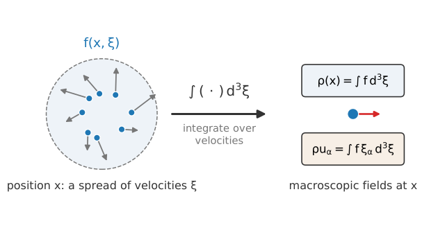
Macroscopic fields are moments of the distribution. At a position x the gas is a spread of molecular velocities xi; integrating f over xi gives the density rho(x), and weighting by xi gives the momentum.

The second moment (weight by \(\xi_\alpha \xi_\beta\)) carries the momentum flux. Splitting the molecular velocity into the mean plus a fluctuation, \(\xi_\alpha = u_\alpha + c_\alpha\), separates this flux into the momentum carried by the bulk motion and the momentum carried by the chaotic thermal motion [2][1]:

(4)\[ \Pi_{\alpha\beta}(\boldsymbol{x}, t) = \int f\, \xi_\alpha \xi_\beta\, \mathrm{d}^3 \xi = \underbrace{\rho\, u_\alpha u_\beta}_{\text{convective}} + \underbrace{\int f\, c_\alpha c_\beta\, \mathrm{d}^3 \xi}_{P_{\alpha\beta}} \]

where the cross terms drop out because the fluctuation has zero mean by construction, \(\int f\, c_\alpha\, \mathrm{d}^3 \xi = 0\). The fluctuation flux \(P_{\alpha\beta}\) is the momentum flux seen by an observer moving with the flow, and it splits into an isotropic and an anisotropic part:

(5)\[ P_{\alpha\beta} = \underbrace{p\, \delta_{\alpha\beta}}_{\text{isotropic: pressure}} + \underbrace{\sigma_{\alpha\beta}}_{\text{anisotropic: viscous stress}} \]

The isotropic part is fixed by the trace and is, by definition, the (mechanical) pressure:

(6)\[ p = \tfrac{1}{3} P_{\gamma\gamma} = \tfrac{1}{3} \int f\, c_\gamma c_\gamma\, \mathrm{d}^3 \xi \]

and the traceless remainder is the viscous stress:

(7)\[ \sigma_{\alpha\beta} = \int f\left(c_\alpha c_\beta - \tfrac{1}{3}\, c_\gamma c_\gamma\, \delta_{\alpha\beta}\right) \mathrm{d}^3 \xi \]

This is the single most important idea to carry forward. Pressure and stress are not separate fields that have to be modeled; they are moments of the same \(f\). The Lattice Boltzmann Method inherits this directly: density, velocity and stress all come from sums of the discrete populations, with no pressure-Poisson equation to solve. The macroscopics page makes this concrete for the discrete case.

Key idea: no pressure equation

Pressure and stress are moments of the same \(f\), so the lattice method gets them for free from sums of the populations, with no pressure-Poisson equation to solve. The same moment structure reappears throughout the chapter: the discrete equilibrium and non-equilibrium moments of the populations (see collision operators) are nothing but the discrete versions of the integrals above.

The Maxwell-Boltzmann equilibrium

Left to themselves, with no walls or forces driving them, molecules collide until the velocity distribution settles into a unique statistical state: thermodynamic equilibrium. For a gas this state is the Maxwell-Boltzmann distribution, a Gaussian in the molecular velocity centered on the local mean flow \(u_\alpha\) [2][1]:

(8)\[ f^{\mathrm{eq}}(\rho, \boldsymbol{u}, \boldsymbol{\xi}) = \rho \left(\frac{1}{2\pi R T}\right)^{3/2} \exp\!\left[-\frac{(\boldsymbol{\xi} - \boldsymbol{u})^2}{2 R T}\right] \]

where \(R\) is the specific gas constant and \(T\) the temperature. Three features matter for everything that follows:

• It is centered on \(\boldsymbol{u}\). The most probable molecular velocity is the bulk velocity; the spread around it is the thermal agitation.

• Its width is set by the temperature. The variance \(R T\) is, physically, the square of the speed of sound. This is the origin of the constant \(c_s\) that pervades the Lattice Boltzmann equations.

• Its moments are exactly the equilibrium macroscopic quantities: integrating (8) as in (2), (3) and (4) returns \(\rho\), \(\rho u_\alpha\), and an isotropic stress \(\rho R T\, \delta_{\alpha\beta}\), i.e. the ideal-gas pressure with no viscous part.

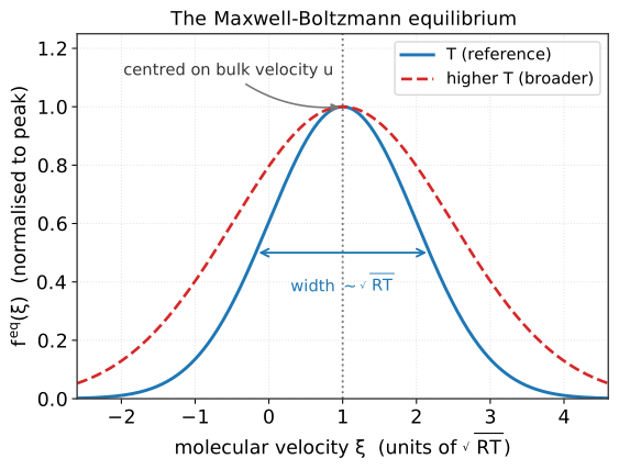
The Maxwell-Boltzmann equilibrium distribution: a Gaussian in molecular velocity centred on the local bulk velocity u, with a width set by the temperature. Raising T broadens it. The lattice Boltzmann method keeps only the low-order moments of this shape.

That last point is the bridge to the discrete method. Because \(f^{\mathrm{eq}}\) is a Gaussian whose only free parameters are \(\rho\), \(\boldsymbol{u}\) and \(T\), it can be expanded compactly in Hermite polynomials and evaluated on a handful of discrete velocities. That expansion, carried out on the next page, is what produces the velocity sets D2Q9, D3Q19 and D3Q27 and their weights.

Mean free path and collisions

Two molecular length and time scales control how fast a gas relaxes toward equilibrium:

• the mean free path \(\ell\), the average distance a molecule travels between collisions;

• the mean collision time \(\tau\), the average time between collisions.

In a flow whose macroscopic features have size \(L\), the ratio \(\mathrm{Kn} = \ell / L\) is the Knudsen number. When \(\mathrm{Kn} \ll 1\), collisions are far more frequent than any macroscopic change, so the gas is driven toward local equilibrium almost everywhere and behaves as a continuum. This is precisely the regime of the incompressible flows Nassu targets, and it is the regime in which the Lattice Boltzmann Method recovers the Navier-Stokes equations (shown explicitly on the Chapman-Enskog page).

The BGK relaxation idea

The full Boltzmann collision term is a complicated double integral over all pairs of colliding molecules. Its essential job, however, is simple to state in words: collisions drive \(f\) toward the local Maxwell-Boltzmann equilibrium. Bhatnagar, Gross and Krook proposed replacing the integral with the simplest operator that does exactly this [3]:

(9)\[ \Omega_{\mathrm{BGK}}(f) = -\frac{1}{\tau}\left(f - f^{\mathrm{eq}}\right) \]

This is a linear relaxation. Wherever the distribution departs from equilibrium, the operator pushes it back at a rate \(1/\tau\). The interpretation of \(\tau\) is direct and physical: it is the relaxation time, of the order of the mean collision time. A small \(\tau\) means very frequent collisions and rapid return to equilibrium; a large \(\tau\) means the flow can sustain large departures from equilibrium for longer.

The departure from equilibrium is not a nuisance to be eliminated. It is exactly what carries the viscous stress: the more the distribution is bent away from the Gaussian by velocity gradients, the larger the viscous momentum transport. The Chapman-Enskog analysis makes this quantitative and shows that the viscosity is set directly by \(\tau\). The Lattice Boltzmann counterpart of that result, the relation between viscosity and the relaxation frequency \(\omega = \Delta t/\tau\), is the cornerstone of how you choose simulation parameters in practice (see the lattice units page).

The three ideas to carry forward

Three threads started here run through the whole chapter: macroscopic quantities are moments of \(f\); equilibrium is the Maxwell-Boltzmann Gaussian; and collisions are a relaxation toward that equilibrium at rate \(1/\tau\). Keep them in mind; everything else is the consequence of discretizing these three ideas.

Next steps

The next page takes the continuous Boltzmann-BGK equation and discretizes its velocity space, producing the discrete populations and the velocity sets used by the solver.

---

[1] (1,2,3,4)

Timm Krüger, Halim Kusumaatmaja, Alexandr Kuzmin, Orest Shardt, Goncalo Silva, and Erlend Magnus Viggen. The lattice Boltzmann method. Graduate Texts in Physics. Springer International Publishing, Basel, Switzerland, 1 edition, November 2016.

[2] (1,2,3)

Sydney Chapman and TG Cowling. The mathematical theory of non uniform gases, cambridge mathematical library. 1970.

[3]

Prabhu Lal Bhatnagar, Eugene P Gross, and Max Krook. A model for collision processes in gases. i. small amplitude processes in charged and neutral one-component systems. Physical review, 94(3):511, 1954.