Poiseuille Pipe (velocity-Neumann)

As for the case of a Poiseuille channel flow, this simulation is used as test for the outlet boundary condition with a fixed pressure. A velocity Bounce-Back BC is used at inlet, to provide an increase of pressure at inlet. The fixed pressure at outlet is meant to avoid a constant increase of the domain average density.

from nassu.cfg.model import ConfigScheme

filename = "validation/analytical/03_poiseuille_pipe_flow/03_poiseuille_pipe_flow.nassu.yaml"

sim_cfgs = ConfigScheme.sim_cfgs_from_file_dct(filename)

The simulation parameters are shown below

import pandas as pd

from nassu.cfg.schemes.simul import SimulationConfigs

dct = {"N": [], "tau": [], "time_steps": []}


def add_to_dict(sim_cfg: SimulationConfigs):
    dct["N"].append(sim_cfg.domain.domain_size.y)
    dct["tau"].append(sim_cfg.models.LBM.tau)
    dct["time_steps"].append(sim_cfg.n_steps)


sim_cfg = next(
    sim_cfg
    for (name, _), sim_cfg in sim_cfgs.items()
    if name.startswith("velocityNeumannPoiseuillePipeMultilevel")
)
add_to_dict(sim_cfg)

df = pd.DataFrame(dct, index=None)

df

	N	tau	time_steps
0	32	0.51	32000

In this case, the IBM domain limits for the \(x\)-direction must be set such that the the body is sufficiently far from domain’s boundaries. Otherwise, numerical instability may be found.

Functions to use for processing of poiseuille pipe.

from typing import Callable

import numpy as np

import nassu.viz as common

common.use_style()


def get_poiseuille_pipe_analytical_func() -> Callable:
    """Poiseuille analytical velocity function

    Returns:
        Callable[[float], float]: Analytical velocity function
    """
    return lambda r: 2 * (1 - r * r)


def get_poiseuille_pipe_numerical_avg_vel(ux_vals: np.ndarray) -> float:
    # Average velocity is ~half the maximun velocity.
    # Numerical integration gives worse results for average velocity
    return np.max(ux_vals) / 2


def get_pos_values_inside_pipe(sim_cfg: SimulationConfigs) -> np.ndarray:
    body = sim_cfg.domain.bodies["cylinder"]
    scale, translation = sim_cfg.domain.export_rescale_components(None, "cylinder geometry", 3)
    lnas = body.get_lnas_rescaled(scale, translation)
    vertices = lnas.geometry.vertices

    x_val = sim_cfg.domain.domain_size.x * 3 // 4 + 2
    z_val = sim_cfg.domain.domain_size.z / 2
    min_y, max_y = (vertices[:, 1].min(), vertices[:, 1].max())
    min_y, max_y = int(np.floor(min_y)), int(np.ceil(max_y))

    p1, p2 = (x_val, min_y, z_val), (x_val, max_y, z_val)
    line = np.linspace(p1, p2, num=max_y - min_y, endpoint=False)
    return line


def get_pos_values_along_pipe(sim_cfg: SimulationConfigs) -> np.ndarray:
    min_x, max_x = 0, sim_cfg.domain.domain_size.x - 1
    y_val = sim_cfg.domain.domain_size.y / 2
    z_val = sim_cfg.domain.domain_size.z / 2

    p1, p2 = (min_x, y_val, z_val), (max_x, y_val, z_val)
    line = np.linspace(p1, p2, num=max_x - min_x, endpoint=False)
    return line


def plot_analytical_poiseuille_pipe_vels(ax):
    x = np.arange(
        -1,
        1.01,
        0.01,
    )
    analytical_func = get_poiseuille_pipe_analytical_func()
    analytical_data = analytical_func(x)
    ax.plot(x, analytical_data, **common.markers.exp_line(linestyle="--"), label="Analytical")

Results

Extract the velocity profile from simulation

import numpy as np
from vtkmodules.util.numpy_support import vtk_to_numpy

extracted_data = {}
array_to_extract = "ux"

export_instantaneous_cfg = sim_cfg.output.exports
macr_export = export_instantaneous_cfg["default"].volumes["default"].inst
data = macr_export.read_export(sim_cfg.n_steps)

pos = get_pos_values_inside_pipe(sim_cfg)

# Sum 0.5 because data is cell data, so it's in the center of the cell
p1 = pos[0] + 0.5
p2 = pos[-1] + 0.5

line = common.create_line(p1, p2, len(pos) - 1)

probe_filter = common.probe_over_line(line, data)

probed_data = vtk_to_numpy(probe_filter.GetOutput().GetPointData().GetArray(array_to_extract))
extracted_data = {"pos": pos, "data": probed_data}

Extract velocity along the pipe

ux_along_pipe = {}

pos = get_pos_values_along_pipe(sim_cfg)
# Sum 0.5 because data is cell data, so it's in the center of the cell
p1 = pos[0] + 0.5
p2 = pos[-1] + 0.5

line = common.create_line(p1, p2, len(pos) - 1)

probe_filter = common.probe_over_line(line, data)

probed_data = vtk_to_numpy(probe_filter.GetOutput().GetPointData().GetArray(array_to_extract))
ux_along_pipe = {"pos": pos, "data": probed_data}

The velocity profile at the end of simulation is compared with the steady state analytical solution below:

import matplotlib.pyplot as plt

fig, ax = common.fig_single()


def normalize_pos(pos):
    # Normalize between -1 and 1
    pos -= pos.min()
    pos /= pos.max()
    pos -= 0.5
    pos *= 2


num_data = extracted_data
num_avg_vel = get_poiseuille_pipe_numerical_avg_vel(extracted_data["data"])
pos_norm = extracted_data["pos"][:, 1].copy()
R = pos_norm.max() - pos_norm.min()
normalize_pos(pos_norm)

ax.plot(
    pos_norm,
    extracted_data["data"] / num_avg_vel,
    **common.markers.sim(shape="o", alpha=0.8),
    label=f"R={R} (avg. {num_avg_vel:.2e})",
)

plot_analytical_poiseuille_pipe_vels(ax)
ax.set_title(f"Poiseuille Pipe\n({sim_cfg.models.LBM.vel_set} {sim_cfg.models.LBM.coll_oper})")
ax.legend()
plt.tight_layout()
plt.show(fig)

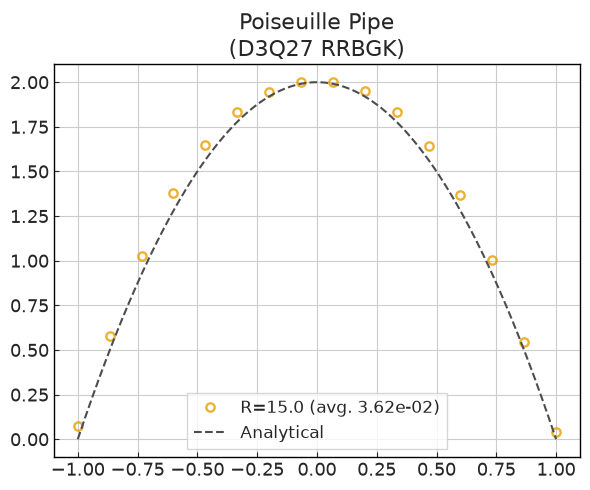
Good agreement was also obtained for this case, with an coherent flow development.

import pyvista as pv

array_to_inspect = "ux"

time_step = macr_export.time_steps(sim_cfg.n_steps)[-1]
xdmf_reader = pv.get_reader(str(macr_export.xdmf_filename))
xdmf_reader.set_active_time_value(float(time_step))
multi_block = xdmf_reader.read()

sliced_blocks = multi_block.slice(
    normal=[1, 0, 0], origin=[3 * sim_cfg.domain.domain_size.x // 4, 0, 0]
)

plotter = pv.Plotter(window_size=(600, 500))
sliced_blocks.set_active_scalars(array_to_inspect)
plotter.add_mesh(sliced_blocks, cmap="coolwarm")
plotter.show(jupyter_backend="static", cpos="yz")

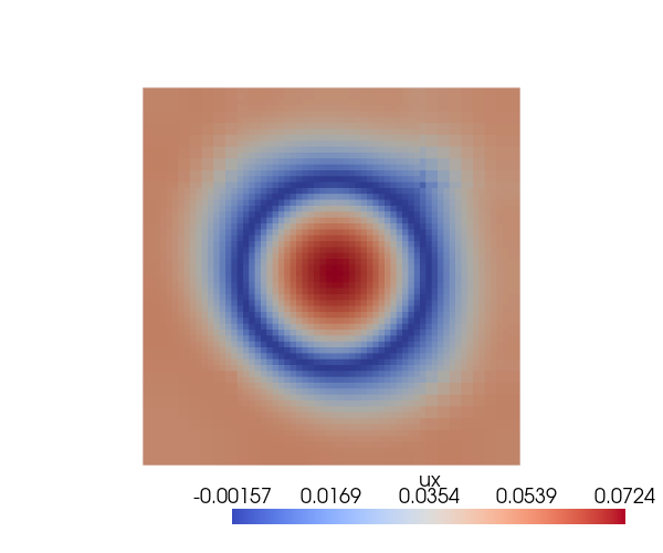
The sectional view of the flow profile shows a axissymmetric flow with a secundary flow ocurring between the IBM body and the boundaries.

import matplotlib.pyplot as plt

fig, ax = common.fig_single()

ax.plot(
    ux_along_pipe["pos"][:, 0],
    ux_along_pipe["data"],
    **common.markers.sim_line(linestyle="--"),
)
ax.set_title(r"$u_x$ at $(x, y=0.5, z=0.5)$")

ax.set_ylabel("$u_x$")
ax.set_xlabel("$x$")
plt.tight_layout()
plt.show(fig)

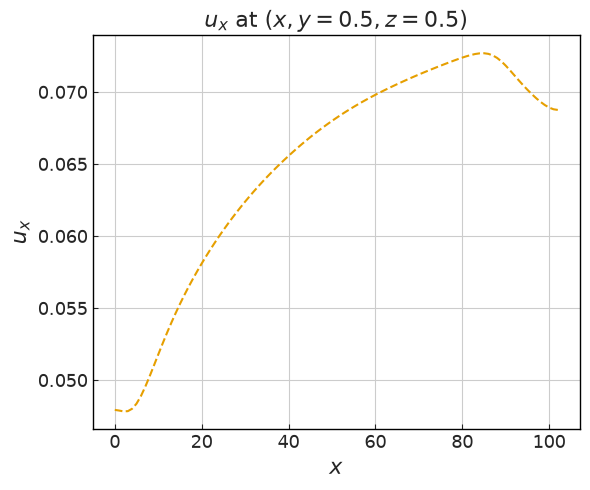
The centerline velocity is shown above. It presents asymptotic decay as for the turbulent channel. However, at the end of IBM domain limits, the flow suffers an expansion and the centerline velocity reduces.

Version

sim_info = sim_cfg.output.read_info()

nassu_commit = sim_info["commit"]
nassu_version = sim_info["version"]
print("Version:", nassu_version)
print("Commit hash:", nassu_commit)

Version: 2.0.1a0
Commit hash: 7c0d788ec9503d2706dadf0db3acd36d61fae57e

Configuration

from IPython.display import Code

Code(filename=filename)

simulations:
  - name: periodicPoiseuillePipeN16
    save_path: ./validation/analytical/03_poiseuille_pipe_flow/results/periodic
    n_steps: 2000
    report:
      frequency: 1000

    data:
      divergence: {frequency: 50}
      exports:
        default:
          macrs: [rho, u, f_IBM, S]
          interval:
            frequency: 0
            lvl: 0
          target:
            volume: {}
          outputs:
            instantaneous: true
        plane_series:
          macrs: [rho, u]
          interval: {frequency: 2000, lvl: 0}
          target:
            planes:
              # Cross-section normal to the streamwise (x) flow at mid-domain.
              # Exported as a triangle surface so ParaView renders the parabolic
              # pipe velocity profile as a plane instead of a point cloud. With
              # min/max omitted the plane spans the full domain; each case below
              # only overrides axis_pos for its own mid-domain x position.
              cross_section:
                axis: x
                axis_pos: 12
                dist: 1

          outputs:
            instantaneous: true
    domain:
      domain_size:
        x: 24
        y: 24
        z: 24
      block_size: 8

      bodies:
        cylinder:
          geometry_path: fixture/stl/basic/cylinder.stl
          small_triangles: add
          transformation:
            scale: [8, 8, 8]
            translation: [-4, 4, 4]

    models:
      precision:
        default: single

      LBM:
        tau: 0.8
        F:
          x: 6.25E-05
          y: 0
          z: 0
        vel_set: D3Q27
        coll_oper: RRBGK

      engine:
        name: CUDA

      IBM:
        forces_accomodate_time: 1000
        body_cfgs:
          default: {}

      BC:
        periodic_dims: [true, false, false]
        BC_map:
          - pos: N
            BC: RegularizedHWBB
            wall_normal: N
            order: 1

          - pos: S
            BC: RegularizedHWBB
            wall_normal: S
            order: 1

          - pos: F
            BC: RegularizedHWBB
            wall_normal: F
            order: 2

          - pos: B
            BC: RegularizedHWBB
            wall_normal: B
            order: 2

  - name: periodicPoiseuillePipeN32
    parent: periodicPoiseuillePipeN16

    n_steps: 8000

    data:
      exports:
        plane_series:
          target:
            planes:
              # Mid-domain x for this domain size; bounds auto-span the full domain.
              cross_section: {axis_pos: 20}

    domain:
      domain_size:
        x: 40
        y: 40
        z: 40
      block_size: 8
      bodies: !not-inherit
        cylinder:
          geometry_path: fixture/stl/basic/cylinder.stl
          small_triangles: add
          transformation:
            scale: [16, 16, 16]
            translation: [-4, 4, 4]

    models:
      LBM:
        F:
          x: 7.8125E-06
          y: 0
          z: 0

  - name: periodicPoiseuillePipeN64
    parent: periodicPoiseuillePipeN16

    n_steps: 32000

    data:
      exports:
        plane_series:
          target:
            planes:
              # Mid-domain x for this domain size; bounds auto-span the full domain.
              cross_section: {axis_pos: 36}

    domain:
      domain_size:
        x: 72
        y: 72
        z: 72
      block_size: 8
      bodies: !not-inherit
        cylinder:
          geometry_path: fixture/stl/basic/cylinder.stl
          small_triangles: add
          transformation:
            scale: [32, 32, 32]
            translation: [-4, 4, 4]
    models:
      LBM:
        F:
          x: 9.76563E-07
          y: 0
          z: 0

  - name: periodicPoiseuillePipeN128
    parent: periodicPoiseuillePipeN16

    n_steps: 128000

    data:
      exports:
        plane_series:
          target:
            planes:
              # Mid-domain x for this domain size; bounds auto-span the full domain.
              cross_section: {axis_pos: 68}

    domain:
      domain_size:
        x: 136
        y: 136
        z: 136
      block_size: 8
      bodies: !not-inherit
        cylinder:
          geometry_path: fixture/stl/basic/cylinder.stl
          small_triangles: add
          transformation:
            scale: [64, 64, 64]
            translation: [-4, 4, 4]
    models:
      LBM:
        F:
          x: 1.22070E-07
          y: 0
          z: 0

  - name: velocityNeumannPoiseuillePipeMultilevel
    save_path: ./validation/analytical/03_poiseuille_pipe_flow/results/velocity_neumann_multilevel

    n_steps: 32000

    report:
      frequency: 1000

    data:
      divergence: {frequency: 1}
      exports:
        default:
          macrs: [rho, u, f_IBM, S]
          interval:
            frequency: 8000
            lvl: 0
          target:
            volume: {}
          outputs:
            instantaneous: true
        plane_series:
          macrs: [rho, u]
          interval: {frequency: 8000, lvl: 0}
          target:
            planes:
              # Cross-section normal to the streamwise (x) flow; bounds omitted so
              # the plane auto-spans the full domain on the in-plane axes.
              cross_section:
                axis: x
                axis_pos: 52
                dist: 1

          outputs:
            instantaneous: true
    domain:
      domain_size:
        x: 104
        y: 32
        z: 32

      block_size: 8
      bodies_domain_limits:
        start: [4, 8, 8]
        end: [88, 40, 40]
        is_abs: true
      bodies:
        cylinder:
          geometry_path: fixture/stl/basic/cylinder.stl
          small_triangles: add
          transformation:
            scale: [8, 8, 8]
            translation: [4, 8, 8]
      refinement:
        static:
          default:
            bodies:
              - body_name: cylinder
                lvl: 1
                normal_offsets: [-2, 0, 2]

    models:
      precision:
        default: single

      LBM:
        tau: 0.51
        vel_set: D3Q27
        coll_oper: RRBGK

      engine:
        name: CUDA

      BC:
        periodic_dims: [false, false, false]
        BC_map:
          - pos: W
            BC: UniformFlow
            wall_normal: W
            rho: 1.0
            ux: 0.05
            uy: 0
            uz: 0
            order: 2

          - pos: E
            BC: RegularizedNeumannOutlet
            rho: 1.0
            wall_normal: E
            order: 2

          - pos: N
            BC: Neumann
            wall_normal: N
            order: 1

          - pos: S
            BC: Neumann
            wall_normal: S
            order: 1

          - pos: F
            BC: Neumann
            wall_normal: F
            order: 0

          - pos: B
            BC: Neumann
            wall_normal: B
            order: 0

      IBM:
        forces_accomodate_time: 1000
        body_cfgs:
          default: {}